MoE Inference Explained: Why Mixture-of-Experts Models Serve Faster

Key Takeaway

• 🧩 The architecture, one line: mixture of experts (MoE) models keep hundreds of specialized sub-networks (“experts”) but route each token through only a few of them — so the model carries the knowledge of a giant while burning the compute of a small one; that asymmetry is exactly what makes MoE inference both fast and hard to engineer.
• 🚦 The serving bottleneck is NOT compute: measurement across MoE serving systems converges on one law — memory bandwidth and expert-routing logistics dominate; the academic MoE inference benchmark work shows throughput converging to the hardware’s bandwidth limit at high FFN sizes regardless of how many experts fire.
• 🛠️ The optimization ledger, mapped: model-level (quantization, expert pruning, speculative decoding), system-level (batching, routing, offloading, CPU-GPU orchestration — Fiddler’s 1.26× single-batch and 11.57× beam-search gains, Lina’s straggler fix), and hardware-level (fused MoE kernels, Grace-Hopper-class bandwidth) — the taxonomy tracks the 2025 ACM survey of MoE inference optimization.
• 💾 Why it matters on your own machine: MoE is why 235B-parameter models run locally on a single high-RAM box — experts stay partly offloaded and the routing keeps active memory tiny; the runner choice (llama.cpp vs vLLM) decides whether those expert swaps help or strangle you.
• 🎯 The takeaway discipline: active-expert management — how many experts stay hot per batch, and which get cached — is emerging as the primary production optimization lever; tune that before buying faster hardware.

Table of Contents

MoE inference is the serving-engineering discipline that turns mixture-of-experts models — the giant-but-sparse architectures behind several of 2026’s most economical frontiers — into services that do not bankrupt their operators. The trick of the architecture (keep all the experts, fire only a few per token) creates a unique serving profile: compute-light in the usual sense, logistics-heavy in ways dense models never face. Benchmarks now measure where MoE serving actually spends its time (mostly waiting on memory bandwidth and expert transfers), and a young optimization field — quantization, expert buffering, fused kernels, CPU-GPU orchestration — is squeezing real multiples out of it. This piece maps the field of MoE inference for practitioners: the architecture’s serving contract, the bandwidth law every MoE system hits, the optimization ledger, and the local-hardware lane where the same physics decides whether a 235B model runs on one box or not.

Who this MoE inference guide is for: anyone serving or self-hosting MoE models — ML engineers tuning vLLM deployments, solo professionals picking between dense and MoE checkpoints, and the enthusiasts who bought a 128 GB Mac specifically to run the big sparse models. The model field guide’s MoE tier named the models; this piece explains the machinery underneath their speed.

MoE inference, defined: the sparse model that serves like a big one

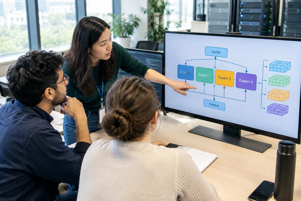
The mixture of experts, precisely: in a mixture-of-experts model, the transformer’s feed-forward layers are replaced by many parallel “expert” FFN blocks plus a router — a small network that, for every token, selects a handful of experts (typically one to eight of dozens or hundreds) to process it. Parameters per token touched: tiny; total knowledge stored: enormous. The DeepSeek-class MoE models and gpt-oss checkpoints this site’s field guide serves from are built exactly this way — sparse FFN layers with routers choosing a few experts each.

Why the architecture matters for serving: the compute-per-token is a fraction of an equivalent dense model’s — the 3-5× serving-speed advantage documented for local MoE checkpoints (and larger commercially) comes from this: fewer layers actually fire per token. The price: ALL the expert weights must live somewhere accessible — a dense 27B and a sparse 235B with the same active-parameter count still differ by 200 GB of resident-or-offloaded memory — and the router’s choices create irregular memory-access patterns dense hardware never planned for. MoE inference is the discipline of managing that gap: big total memory, small active compute, awkward logistics.

The bandwidth law: why more experts stop helping

The measured law: the SC’25 benchmarking work (MoE-Inference-Bench) put the boundary sharply: at larger FFN sizes on H100-class hardware, throughput converges regardless of active-expert count — because memory bandwidth saturation overrides computational parallelism benefits. Once the active-expert working set plus routing overhead exceeds what HBM can stream, adding experts or activations buys nothing; the GPU is bandwidth-limited, not compute-limited. The same benchmark distills a production-level verdict: total parameter budget, not maximum expert count, is what should be optimized — active-expert management is the primary deployment lever.

What the law predicts — and what operators see: batch-size tuning that stops paying beyond a point (the bandwidth ceiling absorbs more traffic without more throughput); the diminishing returns curve on bigger expert counts; the effectiveness of quantization and pruning (they shrink the STREAMED BYTES, which is the binding resource); and why fused MoE kernels (batching many small expert GEMMs into memory-efficient ones) became a default in every serious serving stack. The local case confirms the law: our local-LLM setup guide’s speed-cliff section documents the same physics one scale down — the moment the model’s working set stops fitting GPU memory, per-token speed falls tenfold — and MoE’s entire local-run value is the routing that keeps the hot set small.

The optimization ledger: three levels, mapped

Level 1 — model-level (shrink what streams): quantization (MXFP4 in gpt-oss; the GGUF quant families in local serving — the field guide’s memory-band table carries the sizing math), expert pruning (removing whole experts between uses — intra- and inter-expert pruning both measured in the benchmark suite), and speculative decoding (draft-and-verify flows that sidestep the bandwidth tax on long generations). Level 2 — system-level (move what streams better): batching dynamics (the traffic-shape decisions below), expert buffering and caching (the NeurIPS-2024 optimizations cut activation memory by 79.6% on LM inference at batch 8 by retaining only usefully-hot experts), routing load-balancing (preventing hot experts that create all-to-all imbalance), CPU-GPU orchestration (Fiddler’s placement engine — 1.26× single-batch inference, 1.30× long-prefill, 11.57× beam-search on constrained-GPU MoE setups), and offloading hierarchies (the runner guide’s offload doctrine applies to MoE with expert-level granularity). Level 3 — hardware-level: fused MoE kernels, expert-parallel topologies, and the CPU-GPU bandwidth fixes (Grace-Hopper-class unified memory directly attacks the 12 GB/s transfer bottleneck the NeurIPS work measured on PCIe systems).

How to read the MoE inference ledger: the levels compound, but the binding constraint decides which lever pays — if your serving runs under the bandwidth law (most dense-GPU MoE serving does), Level-1 shrinkage pays most; if expert transfers cross PCIe constantly (small-GPU local or edge serving), Level-2 orchestration pays; if you run multi-node expert-parallel fleets, Level-3 topology dominates. The 2025 ACM survey’s three-level taxonomy (model/system/hardware) is the field’s organizing map, and every serious MoE deployment decision starts by locating itself on it.

The MoE inference batching economics: why MoE loves traffic

The counterintuitive MoE inference fact: MoE models are often CHEAPER at scale than at low traffic — because batching amortizes expert-activation overhead: at batch size 1, each token’s few-expert routing runs with all the fixed costs (router compute, weight staging, kernel launches); at batch 64, one activation serves 64 tokens’ worth of routed computations. The benchmark suite quantifies the shape: active-expert counts interact with batch size nonlinearly — higher batches absorb more active experts before performance degrades, which is why production MoE deployments chase throughput workloads rather than latency-critical single streams.

The practical serving rule, from the interaction: MoE deployments price best under batched, high-traffic serving (chat products, classification fleets, agentic pools) and degrade toward single-stream latency work; dense models hold the single-stream edge. The local-vs-cloud cost piece applies the same shape to provider pricing — the cloud inference economics favor MoE because serving at batch converts sparse compute into real per-token savings — and it is why several frontier labs price MoE-backed product lines below their dense equivalents.

The straggler problem: when routings go bad

The failure mode, measured (Lina, USENIX ATC-23): in distributed MoE serving, expert requests scatter across nodes — and expert popularity is skewed: some experts get most tokens, some get none. The least-popular expert idles up to 29.4% of a batch’s inference time waiting on the popular ones — the batch completes at the PACE OF THE SLOWEST NODE, and naive deployments strand huge bandwidth waiting for stragglers. The paper’s fixes (expert repacking across devices, iterative re-balancing until FFN compute masks the all-to-all, DRAM offloading on overflow) lifted GPU utilization 66.2%→83.4% on 16-expert configurations — representative of the class of fixes: expert PLACEMENT is a serving decision, not a training artifact.

The MoE inference production discipline: routing-aware placement (co-locating co-activated experts), load-balanced routing objectives (the survey tracks global-batch load-balancing methods that keep expert specializations useful), and monitoring that watches per-expert token counts rather than fleet-average numbers. The agent-tools ledger audience will recognize the pattern from fleet management: the tail decides the throughput — treat expert hot-spots as the tail.

MoE inference on your own hardware: the local lane

Why local MoE is suddenly the interesting row: the checkpoint class this site’s local-LLM pieces serve — gpt-oss 20B (MXFP4, ~16 GB), the Qwen MoE checkpoints, DeepSeek-R1’s distilled rows — are all mixtures-of-experts, and the local lane’s flagship claim rides on it: a 235B-parameter MoE runs on high-RAM consumer boxes precisely because experts stay offloaded and routers keep the active set small. The mechanics, from the optimization ledger: the runner keeps the attention layers and hot experts in GPU memory, streams cold experts from system RAM on demand (the expert-buffering problem at household scale — the same 12 GB/s PCIe tax, the same caching logic), and the batch effects differ (chat serving is single-stream — you eat the expert-streaming cost per token, which is exactly the speed-cliff math the local guide prices).

The honest local recommendation stack: local MoE wins when system RAM is abundant (128 GB+ class for the 200B-class models) and traffic is tolerant (drafting, batch classification); it loses on single-stream latency versus dense same-active-size checkpoints and on 8-24 GB GPU boxes, where expert streaming strangles — the field guide’s memory bands price every row of that trade-off. The monitoring habit (one command): watch the runner’s offload state (`ollama ps`-style checks per the runner guide) — a MoE model silently running entirely from RAM is the local version of the bandwidth law, and it is the first thing to check when a previously-served model suddenly crawls.

WorldNgayon Insight: the sparse generation is the serving generation

The frontier quietly converged on sparsity for one commercial reason: token economics. Dense scaling bought quality at linear compute; MoE scaling buys comparable quality on flat-or-falling per-token cost — and 2026’s price competition made that trade irresistible (the field guide’s cost section carries the per-token math). The serving-era consequence: the skills that mattered in the dense era (raw FLOPs, GPU selection) now matter less than the sparse era’s skills — expert caching, routing health, batch-shape economics, offload hierarchies. The engineering field named it in the benchmark’s verdict: active-expert management is the primary production optimization level. The professionals fluent in it are this cycle’s scarce hire — and the knowledge transfers from hyperscale fleets to one-box local runs: the bandwidth law does not care where the model lives.

Verdict: route first, buy bandwidth second

MoE inference, settled: the architecture serves the knowledge of a giant on the compute of a small one, and its speed is governed by memory bandwidth and logistics, not compute size. The optimization ledger runs three levels (model/system/hardware); the benchmark law says shrink the streamed bytes before adding parallelism; the batching economics reward MoE under traffic and punish it on single-stream latency; the straggler problem — skewed expert popularity — is a placement and routing discipline; and locally, the same physics prices every MoE checkpoint by whether its hot set fits your GPU. Route first, buy bandwidth second — the serving playbook of the sparse generation.

Financial Disclaimer

This article is editorial analysis of publicly reported technical and market information, not investment or financial advice, and no outcome is promised. Technologies, vendor claims and market projections change frequently; verify with the named sources. Technology markets carry substantial risk.

Sources on the record: the ACM Computing Surveys MoE-optimization survey · the arXiv MoE-optimization survey preprint.

One measurement caution closes the field map: benchmark numbers travel badly across hardware. The gains cited throughout this piece were measured on specific clusters – Fiddler on CPU-GPU orchestration rigs, Lina on InfiniBand A100 fleets, the benchmark suite on H100s – and your serving environment reproduces none of them exactly. The honest use of the published numbers is directional: they tell you WHICH LEVER to pull first (the bandwidth law says shrink the streamed bytes; the straggler data says watch routing health; the batching curves say price your traffic shape). Measure your own serving before and after any change – the MoE inference stack rewards the operator who instruments first and tunes second.

@online{agron2026moeinference,
  author       = {Agron, Edmon},
  title        = {{MoE Inference Explained: Why Mixture-of-Experts Models Serve Faster}},
  year         = {2026},
  date         = {2026-10-31},
  organization = {WorldNgayon},
  url          = {https://worldngayon.com/moe-inference/},
  urldate      = {}
}

TY  - ELEC
AU  - Agron, Edmon
TI  - MoE Inference Explained: Why Mixture-of-Experts Models Serve Faster
T2  - WorldNgayon
PY  - 2026
DA  - 2026/10/31/
UR  - https://worldngayon.com/moe-inference/
Y2  - 
ER  -